Más cálculos de notas con rúbricas

🔝To translate this blog post to your language, select it in the top left Google box.

¡¡¡ Este es mi regalo para el día de los Reyes Magos !!!

De vuelta con las rúbricas

He recibido varios comentarios en los que me piden que explique:

Cómo añadir una fila más al ejemplo de un cuaderno de rúbricas.

La versión original la publiqué hace dos años aquí:

• Cálculo de notas con rúbricas | #ExcelPedroWave

Si alguien piensa que es fácil añadir una fila más a las rúbricas, ¡está muy equivocado!

Mi mejor regalo de Reyes Magos

Es como un encaje de bolillos, similar al que hacíamos mi hermano, q. e. p. d., y yo de niños construyendo maquetas de barcos con palillos, siguiendo muchos pasos hasta alcanzar el resultado final. El mejor regalo que nos traían los Reyes Magos eran cajas de palillos y pegamento con los que podíamos construir cualquier cosa...

¡Es lo mismo que hago ahora con Excel, que puedo construir cualquier cosa: hojas; libros; plantillas; prototipos o maquetas!

Cómo añadir una fila más a las rúbricas

El resultado de añadir un fila más al cálculo de notas con rúbricas se puede ver en esta imagen:

¡No es tan fácil como agregar una fila más en una tabla de Excel!

Para añadir la nueva fila 13 de la imagen, con un nuevo criterio, hace falta:

• Crear un nuevo criterio en la celda B13.
• Cambiar los porcentajes de los criterios en la columna C.
• Crear el Grupo 5 de botones de opción.
• Crear 4 nuevos botones de opción.
• Vincular los 4 botones a la misma celda oculta en O13.
• Ampliar los formatos condicionales a la fila 13.
• Calcular la nota del nuevo criterio en la celda M13.
• Modificar las fórmulas de las celdas M2 y M3 para calcular la nota final.
• Editar el texto de las celdas: E13, G13, I13 y K13.

Son suficientes cambios para que, hasta un usuario intermedio de Excel, no logre conseguir llevar a cabo satisfactoriamente este encaje de bolillos.

Cuando publiqué los pasos a seguir por primera vez, una lectora me contestó lo siguiente:

En el paso de copiar botones ya me pierdo... pues no me aparece la opción... sería posible facilitarte mi email por privado y que me facilites la plantilla con una fila más? le estaría muy agradecida. Un saludo

Le contesté lo siguiente:

No es posible que envíe plantillas a correos privados, pues mi meta es compartirlas con mis lectores anónimos. Tendrás que esperar a ver esta plantilla en mi blog, pues pienso publicarla con una fila más, como deseas...

Pasos para añadir más criterios

Pero antes de que descargues la plantilla, al final de este artículo, sería interesante que aprendas a añadir una fila más a la rúbrica, por si algún día quieres añadir más criterios. 

Estos son los 31 pasos a seguir para añadir una fila más a la rúbrica de la hoja 'Cuaderno':

1) Desproteger la hoja desde la cinta de opciones: Revisar > Desproteger hoja

2) En la cinta de opciones: Inicio > Buscar y seleccionar > Panel de selección...

3) Seleccionar: Grupo Botones

4) En la cinta de opciones: Formato de forma > Agrupar > Desagrupar

5) Presionar la tecla de escape: <Esc>

6) Seleccionar la fila 13.

7) Insertar 2 filas.

8) Seleccionar las filas 9 a 11.

9) En la cinta de opciones: Inicio > Portapapeles, seleccionar la brocha: Copiar formato

10) Pegar el formato en las filas 11 a 13.

11) Mover hacia abajo la imagen: Copyright

12) Seleccionar en la cinta de opciones: Inicio > Buscar y seleccionar > Panel de selección...

13) Copiar Grupo 4 y Opción Botón 44, 43, 42 y 41.

14) Pegarlos en la fila 13.

15) Cambiarles el nombre: Grupo 5 y Opción Botón 54, 53, 52 y 51.

16) Mover el grupo y los 4 botones pegados hacia el final en el Panel de selección...

17) Presionar la tecla de escape: <Esc>

18) Ocultar: Grupo 1 a 5.

19) Copiar la celda M11 en la celda M13.

20) Cambiar el porcentaje al 20% en las celdas: C5, C7, C9, C11 y C13.

21) Editar la fórmula del formato condicional de la celda C13: =O(REDONDEAR(SUMA($C$5:$C$13);2)<0,99;REDONDEAR(SUMA($C$5:$C$13);2)>1)

22) Seleccionar el Opción Botón 54

23) Hacer clic derecho en la selección y elegir: Formato de control...

24) Vincular con la celda: $O$13 y presionar el botón: Aceptar

25) En el Panel de selección, presionar el botón: Ocultar todo

26) Editar el texto en las celdas: B13, E13, G13, I13 y K13.

27) Ocultar: Grupo 1 a 5.

28) Modificar la fórmula de la celda M2: =10*SUMA($M$5:$M$13)/($E$3*CONTAR.SI($C$5:$C$13;">0"))

29) Modificar la fórmula de la celda M3: =SUMA($M$5:$M$13)&"/"&$E$3*CONTAR.SI($C$5:$C$13;">0")

30) Proteger la hoja.

31) Guardar el libro con otro nombre.

¡¡¡ Bien hecho si has llegado hasta aquí !!!

Descarga las rúbricas mas recientes

Descarga la versión 2, con una fila más en el cuaderno de rúbricas con un nuevo criterio, desde este enlace:

• Sites Google Drive: Calcular notas con rúbricas - PW2.xlsx

Abre el archivo y presiona el botón: Habilitar edición cuando aparezca el aviso de VISTA PROTEGIDA.

El archivo es compatible con versiones desde Excel 2010, tiene las hojas protegidas sin contraseña para evitar que los usuarios alteren las fórmulas, y no contiene macros.

ATENCIÓN: Se puede modificar este libro de Excel respetando esta licencia:

Creative Commons — Atribución-NoComercial-CompartirIgual-No portada — CC BY-NC-SA 4.0

¡¡¡ Que los Reyes Magos cumplan todos tus deseos !!!

¡¡¡ Aunque no seas monárquico !!!

Animated Olympic Chart in Excel

🔝To translate this blog post to your language, select it in the top left Google box.

This article is dedicated to today's opening of the Paris 2024 Olympic Games.

This month of July I've written a couple of articles in Spanish about charts with the image of the Eiffel Tower and the Olympic rings, which you can read here:

• Search results for Eiffel | #ExcelPedroWave

I now publish the English version of my Animated Olympic Chart in Excel, with the following features:

1) The animation starts/stops by clicking on the Olympic torch.

2) The animation depicts the Eiffel Tower's 27-month construction period.

3) Shows the 5 interlocking Olympic rings, with one color per continent.

4) The 3 Olympic Games held in Paris took place in 1900, 1924, and 2024.

5) The Olympic rings move automatically.

6) Manual movement of the Olympic rings with a vertical scrollbar.

7) Animation translation into 6 languages: Spanish, English, French, Italian, German and Portuguese.

8) Animation speed control with a dropdown in cell Z5: 1 to 9, minimum to maximum speed respectively. (*)

9) Version compatible with all desktop versions of Excel. (*)

The last two features, marked with (*), are new improvements to this version of the Animated Olympic Chart in Excel.

Download the Animated Olympic Chart

The Animated Olympic Chart is compatible with all desktop versions of Excel, from Excel 2010 to Excel for Microsoft 365.

Download the latest version from one of these links:

• Microsoft OneDrive: Animated Olympic Chart - PW1.xlsm

• Sites Google Drive: Animated Olympic Chart - PW1.xlsm

Macros in the downloaded file are blocked by default. To unlock macros you must modify the File Properties following these instructions:

• Macros from the internet are blocked by default in Office - Microsoft 365 Apps | Microsoft Learn

Open the file and press the button: Enable Editing when the PROTECTED VIEW prompt appears.

Press the button: Enable Content when the WARNING appears SECURITY Macros have been disabled or part of the active content.

Sheets are protected without password, so you can study the formulas and analyze the chart protected by the macro: ProtectChart.

ATTENTION: You can modify this Excel workbook respecting this license:

CC BY-NC-SA 4.0 Deed | Attribution-NonCommercial-ShareAlike 4.0 International | Creative Commons

Video with the Animated Olympic Chart

The video presents the Animated Olympic Chart, ideal for those without a compatible Excel version or who prefer not to download the file.

This summer we will find out the number of Olympic medals 🥇🥈🥉 that athletes get in Paris.

Salary Data Comparator

🔝To translate this blog post to your language, select it in the top left Google box.

Types of data professionals

I have designed this Salary Data Comparator to know the salary of data professionals:

• Data Analyst: Helps make decisions by analyzing, cleaning and transforming data.

• Data Scientist: Knows statistics, big data, algorithms, scientific computing, etc.

• Data Engineer: It is capable of designing databases, analyzing and processing segmented information (data pipeline), etc.

• AI/ML Engineer: Artificial Intelligence (AI) and Machine Learning (ML) Engineer.

In this animated image I compare the salaries in the USA vs Italy of these 4 types of data professionals.

I show the salary range between the minimum and the maximum salary, with the option of also showing the average salary, which is the most common among professionals in the two chosen countries.

Who gave me the idea of ​​comparing salary data?

The Italian Roberto Mensa is the greatest charts expert I know, so he has managed to be Microsoft Excel MVP.

His specialty is "doing the impossible" with Excel charts, and he demonstrates it in his Gallery:

• E90E50charts - Excel Charts Gallery (google.com)

A few weeks ago he published a radar chart with the Types of Data Professionals:

• Types of Data Professionals - Radar Chart by roberto mensa | LinkedIn

In addition to the radar chart, with the skills of the 4 types of data professionals, it also represents the popularity of these professionals in a line chart, and the salary range of these 4 professions in a scatter chart, in thousands of US dollars ( k$).

It does not specify whether the salary ranges are worldwide or what country those salaries are from. It is assumed that they are from the United States, since their salaries are considerably high compared to those in European countries.

I have uploaded Roberto's file to my OneDrive cloud with his authorization.

To adjust cloud zoom:

• On your mobile or cell phone, use two fingers on the screen, like you do to enlarge or reduce a photo.
• On the PC, place the cursor inside the search engine and press the <Control> key by turning the mouse wheel.

I have simply made the following changes to the Roberto's salary range chart:

• Salary range with the average salary marked with a diamond 🔶
• Option to show average salary.
• List of countries to compare.
• Selection of one or two countries.
• Labels of the types of professionals to the left of zero salary.
• Salaries in a country or comparator of salaries in two countries.
• Dynamic chart title to show the names of the countries compared.
• Comparator in 6 languages: English, Spanish, French, Italian, German and Portuguese.
• Exchange rate of 3 types of currencies: Euros (€), Pounds sterling (£) and American dollars ($).

Salary comparator data

The first thing I did was obtain the salary range data of the 4 types of data professionals for 9 countries, along with their average salary, and I saved them in a table on the 'Data' sheet:

I have decided to compare the salaries of 7 European countries, Mexico and the United States, to make it more international.

I obtained these annual salary data, in thousands of euros (k€), by asking the AI of Microsoft Copilot on Bing, with some Prompts that I am not going to reproduce here.

The AI ​​responded with salary data imported from various sources in thousands of euros (€), as I requested.

When the currency rate changes, it will be necessary to update it in the cells in yellow background, with the conversion rate from pounds sterling (£) and US dollars ($) to euros (€).

Transformation of salary data

Roberto Mensa's version uses the latest Excel features, such as functions LAMBDA y LET, to obtain the series data from the chart.

The hidden sheet 'Support' contains the formulas for the scatter plot with straight lines and markers, with which the salary ranges are represented. In cell Q2 is the Spilled dynamic array formula with the X values ​​of the series. In cell Q7 is the formula with the Y values ​​of the series.

These formulas are very elegant and complex, since they ensure that the headers with the names of the series and their data are generated with a single formula.

The biggest problem is that using the LAMBDA function limits the chart to the versions of Excel for Microsoft 365 and Excel for the web, so it is not compatible with older versions of Excel.

It also adds a level of difficulty for Excel users who are unaware of these new functions, so there will be few who understand them and even fewer who can modify the functions of cells Q2 and Q7.

I haven't even tried to analyze and understand those formulas! and even less modify them!

Roberto, we need a detailed explanation of those formulas to understand them!

I am in favor of designing spreadsheets compatible with all possible versions of Excel, from Excel 2010 to Excel for Microsoft 365, since my followers are scattered around the world and many do not have the most recent versions of Excel installed. Which forces me to use functions common to all those versions of Excel and check compatibility following these guidelines:

• Worksheet compatibility issues - Microsoft Support

My Salary Data Comparator transforms the data in the hidden 'Auxiliary' sheet.

The pivot table for the A:E columns has the data source in the salary table of the 'Data' sheet.

The pivot table for the M column contains the Average (Yes/No) option.

The auxiliary table of the range G1:K8 are the X values of the scatter chart series, obtained with formulas compatible with the GETPIVOTDATA function, that returns visible data from the dynamic salary table.

The auxiliary table of the range G12:K19 are the Y values ​​of the scatter chart series, obtained with the auxiliary formulas of the range H11:K11 and the value of cell G22, to know if it has been filtered by a single country or by several countries.

Since the ranges H5:K5 and H16:K16 are empty, the straight lines that would join a salary range of the first country to be compared with the salary range of the second country disappear.

The value -50 in cell G11 is the X value of the series labels with the names of the 4 types of data professionals. This way the labels with the low values ​​of the salary ranges do not overlap in the scatter chart!

The chart title is obtained in the G21 and J21 cells.

Salary Data Comparator Languages

In the 'Languages' sheet there are the translations into the 6 languages ​​of this Comparator:

Salary Data Comparator Chart

The Salary Data Comparator is represented in a single XY scatter chart with straight lines and markers.

Salary ranges are represented with 4 data series, one for each type of data professional.

The labels of each type of professional are represented with 4 other data series.

The origin of these series are the auxiliary tables discussed in the previous section.

The range values ​​are united by lines of different color for each of the 4 types of professionals.

The minimum and maximum values ​​are marked with a circle 🔴 and the average values ​​with a diamond 🔶.

The X axis goes from 0 to 250, in thousands of euros (€).

The Y axis goes from 2 to 18 and is not visible. It is used to separate the 8 possible visible salary ranges in the Salary Data Comparator, shown in the following image:

This is the result of comparing the salary ranges of the 4 types of data professionals from 2 countries.

With 3 segmentations you achieve:

• Filter from one to four types of data professionals.
• Filter by one or two countries.
• Filter the option to show (Yes) or not show (No) the average salary.

To change the language of the Salary Data Comparator there is a drop-down list in cell S2.

ATTENTION: After a Language change you must update chart with: Data > Refresh All (Control + Alt + F5)

ATTENTION: Update Currency if the language changes.

Cloud Salary Data Comparator

I've shared the Salary Data Comparator in the Microsoft OneDrive cloud, so it's easy to test even if you don't have Excel installed on your computer.

To adjust cloud zoom:

• On your mobile or cell phone, use two fingers on the screen, like you do to enlarge or reduce a photo.
• On the PC, place the cursor inside the search engine and press the <Control> key by turning the mouse wheel.

NOTICE: The changes you make in my cloud are not saved. To save your changes you have to make a copy in your OneDrive cloud.

Download the Salary Data Comparator

The Salary Data Comparator is compatible with versions from Excel 2010 to Excel for Microsoft 365 and Excel for the web.

Download the latest version from this link:

• Sites Google Drive: Salary Data Comparator - PW1.xlsx

Open the file and press the button: Enable Editing when the PROTECTED VIEW prompt appears.

Sheets and workbook are protected without password, so you can study and analyze the formulas, and view the hidden sheets.

ATTENTION: You can modify this Excel workbook respecting this license:

CC BY-NC-SA 4.0 Deed | Attribution-NonCommercial-ShareAlike 4.0 International | Creative Commons

Other graphs with salary ranges

This page is a classic on salary charts, so I can't help linking it here:

• Salary Chart: Plot Markers on Floating Bars - Peltier Tech

Do you know other types of Excel charts with salary ranges? Comment please!

Cálculo de notas con rúbricas

🔝To translate this blog post to your language, select it in the top left Google box.

Rúbricas en la enseñanza

Hace una semana mi sobrina "la profe" me dijo:

Para calcular las notas uso rúbricas y sería una idea interesante para otro post/vídeo de los tuyos.

En mis años de escuela no se utilizaban las rúbricas, ya que surgieron en los años 80, justo después de que terminara mis estudios.

Por lo que no sabía ni que existían y le tuve que preguntar a mi sobrina:

¿Qué son las rúbricas?

Con sus explicaciones y buscando en Internet llegué a estas conclusiones:

Las rúbricas sirven para corregir los exámenes y los ejercicios de clase y poner notas a los alumnos y las alumnas, pudiendo argumentar con ellos y ellas, y/o con sus progenitores, las calificaciones obtenidas en cada asignatura.

Una rúbrica evalúa un conjunto variado de competencias, por tanto permite hacer una evaluación INTEGRAL de las competencias generales y específicas.

Una rúbrica es, desde el punto de vista del formato, una TABLA.

Me quede con esta última frase y me dije que, siendo una tabla, podría rellenarse con Excel, ¡como no!

Para saber más sobre el uso de rúbricas en la enseñanza, lee aquí:

Rúbrica (docencia) - Wikipedia, la enciclopedia libre

Ejemplos de rúbricas

Mi sobrina me pasó dos imágenes con ejemplos de rúbricas, y con ellas he creado estos dos modelos de rúbricas, que se parecen a las tablas de Excel pero que no son tablas:

Como me dijo mi sobrina hablando de la APP que emplea para calcular notas con rúbricas:

Por ejemplo puedo asignar porcentajes a diferentes elementos y una nota a cada uno y se ve así de bonito, con colores pero también te calcula directamente la nota.

He intentado hacer lo que me dijo usando Excel, según estas especificaciones:

• En la columna de la izquierda se escriben los criterios a evaluar, según unos porcentajes.

• En la fila superior se especifica el desempeño con una puntuación y remarcado en distintos colores, por ejemplo: Muy bien; Bien; Regular; Pobre.

• La matriz de criterios y desempeño se puede detallar.

• Cuando se hace clic en un elemento de la matriz, queda anotada la nota para el criterio de esa fila.

• En cada fila debe hacerse clic en un elemento del desempeño, para obtener su nota.

• Se calcula la nota de la rúbrica teniendo en cuenta los porcentajes de cada criterio y las notas por cada desempeño.

Cómo marcar elementos en las rúbricas

Lo interesante era conseguir marcar un elemento de la matriz, para poder asignar una nota a cada criterio de la rúbrica.

Otra condición de mi sobrina es que se hiciera sin macros VBA, por una razón que explico en la posdata de este artículo.

Solución adoptada:

Para conseguir marcar un elemento de la matriz he tenido que insertar tantos Botones de opción como elementos de la matriz, agrupados en cada fila con Cuadros de grupo, lo que permite hacer clic en ellos para marcar la nota de cada criterio de la rúbrica.

Si no sabes insertar esos controles de formulario, leyendo estos dos artículos aprenderás:

• Agregar una casilla o un botón de opción (controles de formulario) - Soporte técnico de Microsoft

• Agregar un cuadro de grupo o un marco a una hoja de cálculo - Soporte técnico de Microsoft

Y viendo esta imagen se entenderá perfectamente:

TRUCO: Lo que no se ve en la imagen es que los botones de opción cubren su celda y la celda contigua a la derecha, con lo que haciendo clic en cualquiera de las dos celdas se marca la opción seleccionada.

En el ejemplo de la imagen, para la PRESENTACIÓN de la fila 5, como está seleccionado el botón de opción en D5, su celda vinculada es O5 (la columna O está oculta) a la que le asigna el valor 4. Con formatos condicionales se cambia el color de la celda E5. Con una fórmula se calcula la nota en la celda M5. Lo mismo se hace para cada uno de los 16 botones de opción.

El valor de los botones de opción depende de las columnas:

1. Para las columnas J y K.
2. Para las columnas H e I.
3. Para las columnas F y G.
4. Para las columnas D y E.

Así se consigue en la imagen anterior marcar:

• PRESENTACIÓN: Muy bien con un 4 de nota.
• ORGANIZACIÓN: Bien con un 3 de nota.
• CONTENIDOS: Bien con un 3 de nota.
• AUTOCORRECCIÓN: Pobre con un 1 de nota.

Segunda rúbrica para valorar el nivel de inglés

En esta otra imagen aparece la segunda rúbrica de ejemplo.

Esta rúbrica sirve para valorar expresiones escritas en inglés.

ATENCIÓN: Las notas de desempeño pueden ser decimales modificables. Por ejemplo: "Very good" con 1,5 de nota.

Se pueden guardar diferentes hojas para diferentes unidades evaluadas de cada alumno.

También se pueden añadir comentarios para cada criterio de evaluación a la derecha de su nota.

Vídeo explicando las rúbricas

En este video explico cómo he hecho la calculadora de notas con rúbricas.

Selecciona los subtítulos en tu idioma para entender el vídeo.

Descarga las rúbricas de ejemplo

El archivo es compatible con versiones a partir de Excel 2010, tiene las hojas protegidas sin contraseña, para que los usuarios no destrocen las fórmulas, y no contiene macros.

Descarga la versión 1.2 desde este enlace:

• Sites Google Drive: Calcular notas con rúbricas - PW1.xlsx

Actualización: 8 de noviembre de 2025

Descarga la versión 2, con una fila más en el cuaderno de rúbricas con un nuevo criterio, desde este enlace:

• Sites Google Drive: Calcular notas con rúbricas - PW2.xlsx

Actualización: 22 de abril de 2026

Descarga la versión 3, con una columna más en el cuaderno de rúbricas, desde este enlace:

• Sites Google Drive: Calcular notas con rúbricas - PW3.xlsx

Abre el archivo y presiona el botón: Habilitar edición cuando aparezca el aviso de VISTA PROTEGIDA.

Posdata

Cuando compartí estas rúbricas con mi sobrina, me dijo:

Tío, ¿y no se podría compartir en la nube de Microsoft OneDrive al no incluir macros?

Y le tuve que contestar:

Sobrina, ¡Excel para la Web no es compatible con los botones de opción!

AVISO para navegantes y para mi sobrina:

En un próximo artículo podrás ver una rúbrica en Excel funcionando en la nube:

• Calcula tu nivel de Excel | #ExcelPedroWave

¡Es una calculadora de tu nivel de Excel sin salir de mi blog!

AVISO para maestros y profesores:

Con rúbricas es imposible detectar si los alumnos han cometido fraude al entregar trabajos generados por ChatGPT, lo que convertirá a las rúbricas en evaluadoras de la Inteligencia Artificial.

Posdata: Este artículo ha sido generado sin la ayuda de ChatGPT ni ninguna otra IA.

How to convert units of measurement

In Excel there is a very useful function, little known and less used:

CONVERT function - Microsoft Support

With the CONVERT function you can convert some units into other units of the same measure, which is very useful for physicists, chemists, mathematicians, engineers, science students or any Excel user who needs to convert units of measurement.

For example, to convert 1 statute mile to kilometers, the following formula is used:

=CONVERT(1,"mi","km")

Where the first argument is the numeric value to convert, a 1 in the example, the second argument is the abbreviation for miles "mi" and the third argument is the abbreviation for kilometers "km".

Since you have to know the abbreviations for the units of measurement to edit the arguments, I prefer to do it with an Excel workbook that I have prepared to automatically convert some units of measurement into others.

In this measurement converter there are 3 data segmentations:

1. Measurements: to select a measurement type: Area, Distance, Energy, Force, Information, Magnetism, Power, Pressure, Speed, Temperature, Time, Volume (or liquid measure), Weight and mass.
2. Prefix: to select the prefix of the measurement unit, for example: kilo, which is the multiple of a thousand. The equal sign (=) indicates that there is no prefix, so the unit is worth.
3. Units: to select the type of unit depending on the type of measurement.

A numerical value is entered in cell K2 and a table in the range K4:L28 is obtained with the conversion of all the units of the selected measure.

To obtain a certain unit of measurement, its prefix is entered in cell M3, and its type of unit in cell N3, with which the conversion is obtained in L2.

In the range M4:M28, the converted units are obtained with the cell prefix M3.

The abbreviations for each conversion are listed in the range N4:N28, separated by hyphens if there is more than one abbreviation, for conversion of units of measure.

In some of the sheets with tables of units I have edited column D with the abbreviations that do work when converting... I may have left some without adding.

Please tell me if you find any errors in the conversions, so I can correct them as soon as possible...

Convert units of measurement in the cloud

Try converting measurements without the need for Excel and without leaving this page.

When you change the type of measurement you must click on the first of the 4 buttons at the bottom right to: Update all data connections

To adjust the zoom of the embedded book:

• On the mobile or cell phone, use two fingers on the screen, as you do to enlarge or reduce a photo.
• On the PC, place the cursor inside the browser and press the <Control> key while turning the mouse wheel.

Download the measurement converter

Download version 1.0 from this link:

• Sites Google Drive: Convert measurements - PW1.xlsx

This file is compatible with Excel 2016 and higher versions, since it uses:

Dynamic array formulas and spilled array behavior - Microsoft Support

Open the file and press the button: Enable editing when the PROTECTED VIEW notice appears.

Press the button: Enable content when the SECURITY WARNING appears.

The sheets are protected without a password, so you can study and analyze the formulas. You can even modify this workbook as long as you respect this license:

 

Creative Commons — Attribution-NonCommercial-ShareAlike 3.0 Unported (CC BY-NC-SA 3.0)

In the downloaded file you can also analyze the queries in Power Query, with which I have downloaded the measurement unit tables from this web page:

CONVERT function - Microsoft Support

Video-tutorial on how to convert measurements

In this video-tutorial I explain how to convert units of measurement in Spanish.

Select the captions in your language to understand the video-tutorial.

What other conversions between units of measurement would you add?

Tell me and I'll include it in a future version.

My new Excel calculator

🔝To translate this blog post to your language, select it in the top left Google box.

NOTICE: This calculator is designed for educational purposes and personal use. It is not a professional calculator and is provided “AS IS”, without guarantees or responsibilities on the part of the author of this blog. This means that the user assumes all risks associated with the use of this calculator.

My new calculator

My new Excel calculator is based on one I made 12 years ago.

In these two articles I explain the most relevant characteristics of the old calculator, that will help to understand how the new calculator is made:

Calculating minds | #ExcelPedroWave

How to make Excel calculators | #ExcelPedroWave

This last article is in the TOP 5, since it has received more than 31,000 visits, being the fourth of the most visited articles on my blog.

This is the image of my new calculator made in Excel. If you want one, download it below.

Calculator features

The main features of this new calculator made in Excel are:

A) The pressing of the keys by 3 methods:

1) Using the virtual keyboard, being unchecked the Tooltips, a macro is called that detects the key being pressed. It is the elementary method, since all the keys call the same macro.

2) Using the virtual keyboard, being checked the Tooltips, creating the keyboard adds a different hyperlink for each key, using the method: Hyperlinks.Add. It is a more sophisticated method, since each key has a cell associated with it, that is selected with the hyperlink, and the selected cell change event launches the macro that detects the key pressed.

3) Using the physical keyboard, by pressing keys shown in parentheses when you hover over a key, bringing up the information in a Tooltip. For example, with the key 10^x it appears: Ten raised to x (SHIFT+X), so the physical key is the uppercase X. It is the most elaborate method, since a macro has been created for each key, which is called with the method: Application.OnKey

B) The dynamic creation of the calculator keys in 3 cases:

1) When changing the type of calculator, the actual keys are deleted and the new keys of the selected calculator are created. Initially there are 8 calculators in addition to the number 0 that serves as a presentation and help.

2) By checking or unchecking Tooltips, because it is necessary to create or eliminate the hyperlinks of each key.

3) When switching languages, if are checked the Tooltips, because the hyperlinks of each key must be created in the selected language.

C) Customizing calculator keys and recording a new one in 5 steps:

1) Select one of the existing calculators.

2) Disable the physical keyboard to be able to clear the keys with the key: Delete

3) Select and delete the keys that will not appear in the new calculator.

4) Change the size and position of customized keys.

5) Save the new calculator by typing a descriptive name.

D) The 8 features that make this new version of my calculator unique:

1) It is made in Excel with VBA macros, being compatible with desktop versions, from Excel 2010 to Excel for Microsoft 365.

2) Calculation results are viewed in a seven-segment display, being able to easily choose its color, by clicking on one of the colors in row 1.

3) You can see how each key is dynamically created when you change the calculator type, by checking: Floating.

4) The calculator is translated into 6 languages, being able to add more languages.

5) It is a touch calculator, if the screen is touch screen, being able to hide key groups by clicking on the below keys.

6) With 4 new keys to change the Zoom, making the calculator bigger or smaller.

7) With a new date and time key, with the year represented by: yyyy, in 3 different date formats:

• With the year ahead según ISO 8601: yyyy.mm.dd hh:mm:ss
• With the month ahead: mm.dd.yyyy hh:mm:ss
• With the day ahead: dd.mm.yyyy hh:mm:ss

8) It is a scientific calculator in Floating-point arithmetic. It is the main innovation of this new version, since the old calculator only operated in Fixed-point arithmetic, being able to operate the new calculator with very small or very large numbers, like the one that appears in this image:

For numbers in scientific notation the notation E is used, with the same limits of the VBA language for the double data type:

• -1.79769313486231E308 to -4.94065645841247E-324 for negative values
• 4.94065645841247E-324 to 1.79769313486232E308 for positive values

If during any calculation these limits are exceeded, an overflow appears represented as: -E-

If the exponent is positive, it is represented only with the letter E, for example: 4.E3 is equivalent to 4x10^3

If the exponent is negative, it is represented by the letter E and the minus sign, for example: -2.E-3, equals -2x10^-3

Calculator video-tutorial

In this video-tutorial I explain how to use this new calculator.

Select the captions in your language to understand the video-tutorial.

Download the calculator

Download version 5.0 from this link:

• Calculadora Táctil PW5.xlsm

The downloaded file's macros are blocked by default. To unlock the macros you must modify the Properties of the file following these instructions:

• Macros from the internet will be blocked by default in Office - Deploy Office | Microsoft Learn

Open the file and press the button: Enable editing when the PROTECTED VIEW notice appears.

Press the button: Enable content when the WARNING appears SECURITY Macros have been disabled

The sheets are protected without a password and the VBA project is not protected, so you can study and analyze all the code. You can even modify it respecting the license:

Creative Commons — Attribution-NonCommercial-ShareAlike 3.0 Unported (CC BY-NC-SA 3.0)

Feedback of the new calculator

I accept criticism and suggestions if you use and try this new calculator.

To improve this calculator I need to know its bugs, its deficiencies and their possible improvements and, if you give me feedback, I will thank you and I will commit to improve the calculator in future versions during the next few years, I don't expect so many to pass...

And so I finish the series of 4 articles on keyboards and their keys, which I have been publishing for more than a month, and which you can find at this link:

keyboard | #ExcelPedroWave

International Virtual Keyboard in Excel

Download for free at the end of this article the renewed version of the International Virtual Keyboard most complete that exists worldwide made entirely in Excel.

It has all the functions of a few keyboards in a single Graphical user interface. Check it out for yourself!

This virtual keyboard is used for touch screens or as a substitute, if the physical keyboard breaks down. It is also useful for learning and testing various keyboard layout in several languages or in the Dvorak keyboard layout.

You can even create your own keyboard! adding a column in the 'Teclas' sheet.

Background of the Virtual Keyboard in Excel

10 years ago I allowed myself the audacity to modify the original idea of a virtual keyboard of a genius of macros, to make it international.

The idea came from Macro Antonio, a VBA macro expert and friend on Excel forums, who posted his version of a virtual keyboard.

Another of the best Excel forum members I had the pleasure of meeting was verzulsan, who improved the keyboard to repeat the keys in "machine gun" mode, and I made the international version and posted it on my blog:

International virtual keyboard | #ExcelPedroWave

3 weeks ago, a follower of my YouTube channel warned me that the keyboard "only works on old 32-bit systems", which made me review it and I decided to update it, adding the PtrSafe keyword to make it work in 64-bit Excel.

In addition, I myself had written a note in said article: "The Alt key doesn't generate the encoded characters, for example Alt+21 = §"

Then I realized that a follower of the blog had commented 6 years ago that: "Fonts on the page is blank, the fonts are not visible."

Features of the new Virtual Keyboard in Excel

So this International Virtual Keyboard, made entirely in Excel!, incorporates the following new features:

• Compatible with any 32-bit and 64-bit version of Excel.

• Insert symbols and characters with Alt + code, holding down the Alt key while typing the character's decimal code on the numeric keypad, for example Alt+21 = §, explained in: Insert ASCII or Unicode symbols - Microsoft Support

• List the types of text fonts with a dropdown ComboBox that allows you to choose the type of text font: About Microsoft Typography | Microsoft Learn

• New dropdown ComboBox with default Zoom: 100; 125; 150; 175; 200. With the ScrollBar you can continue changing the Zoom.

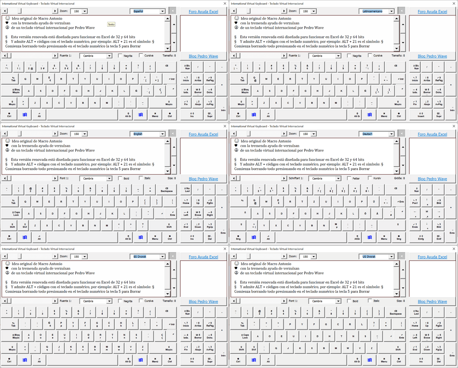
This is how the revamped International Virtual Keyboard looks like with different keyboard layouts in several languages:

Instead of pressing the keys of a physical keyboard, try pressing the keys of this International Virtual Keyboard, with the following functions:

• Design the keyboard doing it entirely in Excel, with a user form: UserFormTeclado built dynamically with VBA macros.

• Translate the keyboard to multiple languages: Español, Latinoamericano, English, Français, Italiano, Deutsch, Português, with the possibility of adding more languages on the 'Teclas' sheet, or even your own custom keyboard.

• Change the layout of the keys: QWERTY, QWERTZ (German), AZERTY (French) and Dvorak keyboard layout in Spanish and English.

• List all Windows text fonts and format the text according to the chosen font.

• Save in the 'Personal' sheet the zoom and the last font, size and text properties.

• Show the symbols of the special keys according to the international standard ISO/IEC 9995.

• Include the special keys: Enter, Tab, Ctrl, Alt Gr, Shift, Caps Lock, Num Lock, Windows key, Menu, Insert, Delete, Home, End, Page Up, Page Down and cursor movement arrows.

• Operate the numeric keypad as a basic calculator.

• Hide or show the numeric keypad.

• Expand the text box with double click.

• Other minor improvements, such as positioning the keyboard on the screen.

• Insert ASCII and Unicode symbols with the key combination Alt + decimal code. This function is explained below.

How to enter special symbols with the Alt key

To enter ASCII and Unicode characters:

• On a physical keyboard, hold down the Alt key and type the decimal code of the ASCII or Unicode character with the numeric keypad. When you release the Alt key, the special symbol appears.

• On the virtual keyboard, press the Alt key (which remains marked), write the decimal code of the ASCII or Unicode character with the numeric keyboard. The Alt key is pressed again and the special symbol appears.

Codes with the Alt key are divided into 3 groups:

• 255 BIOS ASCII codes: Alt+1 to Alt+255

• 128 ANSI codes or Windows Alt codes, with the number 0 in front: Alt+0128 to Alt+0255

• 149186 Unicode codes, with the decimal code of the 1 to 6 digit Unicode character. It should be noted that in this virtual keyboard you cannot enter hexadecimal codes, only decimal codes. For example: Alt+129412 represents the Unicorn symbol: 🦄 (hexadecimal code: 0x1F984)

Some interesting pages about Alt key codes:

Alt code - Wikipedia

List of Unicode characters - Wikipedia

ALT Codes | Windows ALT Key Codes for Characters & Symbols (altcodeslist.com)

Emoji Group: Animal & Nature 🐶 🌻 🐯 (altcodeunicode.com)

Video tutorial of the International Virtual Keyboard

In this video tutorial I explain how to use this International Virtual Keyboard.

Select your language caption to understand the video.

Download the International Virtual Keyboard

Download version 2.0 from one of these links:

• Microsoft OneDrive: International Virtual Keyboard - Teclado Virtual Internacional PW2.xlsm

• Sites Google Drive: International Virtual Keyboard - Teclado Virtual Internacional PW2.xlsm

The downloaded file's macros are blocked by default. To unlock the macros you must modify the file Properties following these instructions:

Macros from the internet will be blocked by default in Office - Deploy Office | Microsoft Learn

Open the file and press the button: Enable editing when the PROTECTED VIEW notice appears.

Press the button: Enable content when the SECURITY WARNING appears Macros have been disabled

The sheets are protected without a password and the VBA project is not protected, so you can study and analyze all the code. You can even modify it respecting these license:

 

Creative Commons —  Attribution-NonCommercial-ShareAlike 3.0 Unported (CC BY-NC-SA 3.0)

Competitors of this Virtual Keyboard in Excel

Compare this keyboard with the Google virtual keyboard on this page:

Try Google Input Tools online

Google's virtual keyboards are built into Google Translate, for example:

Pressing on the keyboard (within the red rectangle) selects the text input tool, for example in English: ⌨️ English; ⌨️ English DVORAK; ✏️ English touch writing.

The main advantage of Google's virtual keyboard over mine is that when you press the physical keyboard keys, it sends the virtual keyboard keys instead.

It will be an issue to consider if I decide to improve these Virtual Keyboard.

In the meantime you can read my previous articles on keyboards and special characters in Excel from here:

keyboard | #ExcelPedroWave